
Appendix to the Radix‑Sort Video
These are the bonus notes about our radix sort video that didn’t fit into the video cut.
More on floats
Try to play with the following widget (clickable squares). It showcases the full minifloat format, including all the technicalities we did not tell you about. Like:
- the number 0 can be represented both as “+0” and “-0”
- the largest exponent “1111” does not encode 15, but infinity, at least when the mantissa bits are “000”. The sign encodes whether it’s +∞ or -∞.
- if the exponent is “1111” and mantissa bits are nonzero, we encode NaN.
- the smallest exponent “0000” includes so-called subnormal numbers – for those, the mantissa XYZ is not interpreted as 1.XYZ, but as 0.XYZ.
- One nice thing about this is that infinities and subnormal numbers still work well with our integer<->float trick! NaNs will end up being even larger than infinities.
- Careful! Our trick does not extend to negative numbers. That’s because integer format handles negative numbers using the two’s complement format (see above widget), while floats simply store the sign as the first bit. It’s not the end of the world though; if we run the unsigned-integer-radixsort for input numbers -2.0, -1.0, 0.0, 1.0, 2.0, we end up with output [0.0, 1.0, 2.0, -1.0, -2.0]. With some small post-processing (split into positive/negative part, reverse negative part and put it to the beginning), we achieve the sorted order.
Float formats
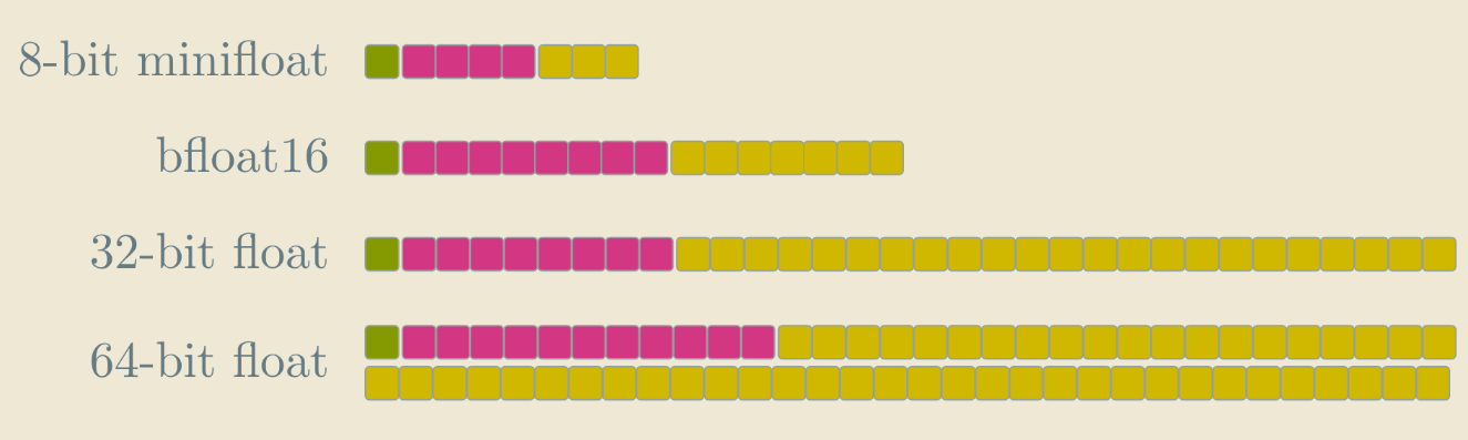
The “minifloat” in the script is mostly a teaching toy; but the same idea scales. Here are the floats you might encounter.
- binary32 (float): 1/8/23. This is the traditional implementation – and often just called “the float”. It’s used in GLSL shaders but in general, I’m not sure how often this is used these days – modern CPUs are optimized well for 64-bit format, while GPUs often use smaller precision.
- binary64 (double): 1/11/52. In C, C++, Java, JavaScript, Python, etc., the literal 1.23 is a double unless you explicitly write 1.23f. If you have to work with floating point numbers, you are entering a huge can of worms. For example, in competitive programming, your program can sometimes give wrong answer just because of the rounding errors made by the float. Using double is not much slower than using floats on CPUs, so it’s pretty much for free.
- bfloat16: 1/8/7. This is popular in deep learning. Neural networks are anyway super noisy by design, so introducing small rounding errors doesn’t really matter
This holds for training and even more so for inference . The nice property of bfloat16 is that it has the same-sized exponent as float, so rounding floats to this format is super fast. There are all kinds of similar formats used for deep learning, see e.g. the wiki page about bfloat16.
How did 1960s machines sort letters?
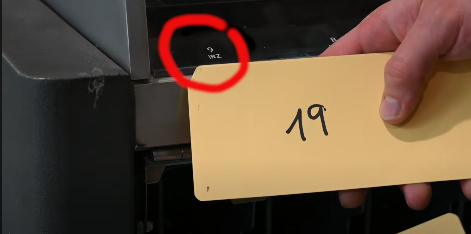
Here’s a fun fact – if you look closely at the IBM 083 machine, you will see that the bucket with 9 also has IRZ written next to it.
Here’s the full table:
| Pocket (digit row) | Label contents |
|---|---|
| 0 | 0 (space) |
| 1 | 1 A J S |
| 2 | 2 B K T |
| 3 | 3 C L U |
| 4 | 4 D M V |
| 5 | 5 E N W |
| 6 | 6 F O X |
| 7 | 7 G P Y |
| 8 | 8 H Q |
| 9 | 9 I R Z |
Do you see what it is for?
.
.
SPOILER
.
.
Yes – the machine can also sort by letters, not just by digits. The only downside is that each letter will need two runs of the machine. In the first run, A, J, S end up in the same bucket. In the second run, only three buckets are needed.
Can we sort strings and black box objects?
In our video, we implicitly claimed that radix sort cannot be used to sort strings. That’s an oversimplification (and we should have probably added some “it depends” symbol to the appropriate table in the video) – the above section shows that the IBM machine was used to literally sort strings. So where’s the catch?
If we simplify and assume that the input text strings are written in ASCII, we could sort them using a radix sort with base $2^7$ – each letter is one digit. The problem is that the time complexity of radix sort then scales with maximum length of the input string $\ell_{max}$ as $O(n \cdot \ell_{max})$. This is OK if we sort surnames (as was done by the machine from 60’s), but if we sort strings of various lengths, some of them potentially long, this scales very poorly.
Similarly, radix sort could be used to sort most objects. Typical comparison functions look like this:
compare(a, b):
if a.x < b.x:
    return true
else if a.x == b.x && a.y < b.y:
    return true
else if a.x == b.x && a.y == b.y && a.z < b.z:
    return true
return false
In this case, we can replace each object a by the corresponding tuple (a.x, a.y, a.z), interpret it as a long integer, and run radixsort. Even more complicated comparison functions will allow embedding like this. The ultimate problem is the same as with strings – radix sorting long integers simply scales poorly, even using our trick of choosing a large base.
Radix tree
A radix tree (or Trie or Patricia trie) is a data structure that is in many ways analogous to radix sort. Instead of storing numbers by comparing them, we partition them into chunks and address our memory by those chunks. See Wikipedia for how that works. As in radix sort, the algorithms will be explained for a small alphabet – like 16 lower-case English letters – but the interesting alphabet is often much larger. For example, an IPv4 address is a sequence of four 8-bit numbers, so choosing the base as 2^8, we may store IP addresses very efficiently in such a way that lookups require just four hops through our radix tree. This is much faster than storing them using the standard binary search tree.
By the way, if we only wanted to store a bunch of IP addresses, we could as well use a simple hash table and not worry about radix trees at all. But the routing tables in routers need to store more complicated information – they don’t store just concrete addresses, but also masks that represent an interval of IP addresses. For each mask, the routing table stores information about where to route an incoming IP address that satisfies this mask. Hence, a hash table is not enough here, we really need a data structure that implements the predecessor operation.
Radix sort complexity and the Word‑RAM model
What’s the time complexity of radix sort? That’s a harder question than it looks like. In classical comparison sorts, computing the time complexity ends up being about counting how many comparisons the algorithm does. For radix sort, we also need to take the bit representation into account.
The standard model in which we analyze algorithms is called Word‑RAM. It’s one of those models that are 1) incredibly important, because technically, most algorithms are analyzed in that model and 2) it’s difficult to find a single definition of it and, in fact, there are several slightly different definitions.
In essence, Word-RAM is essentially the C language model, with the exception that instead of using 32-bit or 64-bit numbers, we just say that there’s a parameter $w$ – word size – such that $w \ge \log n$. We need $w$ to be at least $\log n$ so that our words are large enough to store pointers to the input data. But potentially, $w$ could be larger, it is after all just a parameter.
In this model, we assume that one basic operation with two words (summing them up, multiplying them) takes constant time $O(1)$. On the other hand, iterating over the bits in a word takes non-constant time $O(w)$.
Let’s compute the complexity of radix sort in this model. For integer keys, a radix pass (= 1 bucketsort) with base $B$ costs O(n + B). To cover w bits, we need w / log₂B passes, giving the overall time complexity
The right (theoretical) way to choose $B$ is $B\approx n$. This is sensible – we want the number of buckets to be as large as possible. At the same time, we want the handling of the buckets to be negligible when compared to iterating over the input $n$ numbers. This is also why in the video, we chose $B = 2^{16}$.
Plugging in $B = n$, we get this complexity:
\[T(n,w)=O\!\left(n\cdot\frac{w}{\log n}\right).\]You should think about it like this: Naive radix sort has complexity $O(n \cdot w)$. Using our trick of choosing large base, we can improve $w$ to $\frac{w}{\log n}$. That’s really cool for small $w$s, but it does not change the fact that the time complexity scales with $w$.
In particular, this complexity is slower than the linear time complexity $O(n)$. It is a function that depends on both $n$ and $w$.
- In many practical scenarios (like the scenario in our video), it is reasonable to think of $w$ as $w=O(\log n)$. In that setup, it is actually absolutely correct to claim that radix sort is a linear time algorithm! That may sound weird if you know about the $\Omega(n \log n)$ sorting lower bound, but that lower bound only holds for sorting black-box objects, not integers in the Word-RAM model of computation.
- Other scenarios like sorting long strings correspond to large $w$. So our analysis explains why radix sort is slow there.
Kirkpatrick–Reisch algorithm
There’s a cool algorithm called Kirkpatrick–Reisch sort with even better time complexity. Unfortunately, we ran it
There’s a nice explanation of the algorithm on this great blog. The time complexity of the algorithm is $O(n \log \frac{w}{\log n})$.
Sorting is an open problem!
This is a fine point that did not make it to the video. Although sorting is one of the simplest and most fundamental open problems, we still don’t know whether a linear-time algorithm in the Word-RAM model exists.
The fastest known theoretical algorithms are a bit better than Kirkpatrick–Reisch, but not by much. The complexity of that algorithm is extremely close to being linear, but it’s not $O(n)$. Whether a truly linear-time algorithm exists, for all values of $w$, is an open problem.
I think it’s shocking that even for such a basic problem, and after decades of research, we still don’t know what’s going on!
Random notes
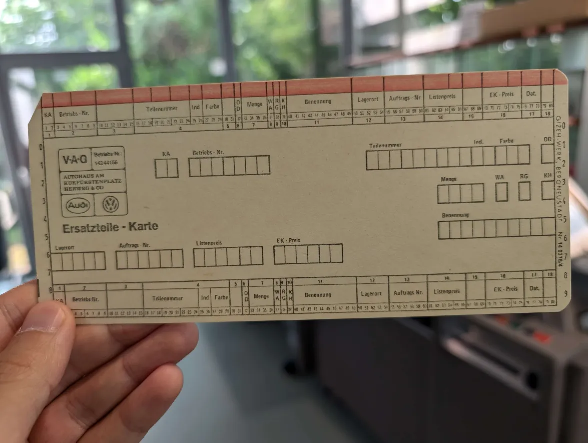
- Correction: when describing a card “storing spare parts for a car company”, we showed just a random card. Here’s the actual one:
- Our implementation of radix sort is also known as American flag sort